Eigenvectors and Eigenvalues
What are Eigenvectors and Eigenvalues. Core concept explained with diagrams, graphs and examples
I am a developer sharing the problems I solve through my blog. Just giving back to the community I learned so much from! Have an amazing day :)
Prerequisites
Linear Transformation and Determinants are the two concepts one needs to be clear about before attempting to learn what Eigenvectors and Eigenvalues are. Once familiar with them, the core concept is pretty simple to grasp.
Core concept
Assuming you are familiar with Linear Transformation and Determinants, let's jump into the core concept of Eigenvectors and Eigenvalues. Consider Matrix A and how it transforms a set of vectors V
$$\begin{array}{l} A = \begin{bmatrix}{} 3 & 1 \\ 0 & 2 \end{bmatrix} \quad V = \begin{bmatrix}{} 1 & -1 \\ 1 & 1 \end{bmatrix} \\ \\ \therefore \quad A \times V = \begin{bmatrix}{} 1 & -2 \\ 2 & 2 \end{bmatrix} \end{array}$$
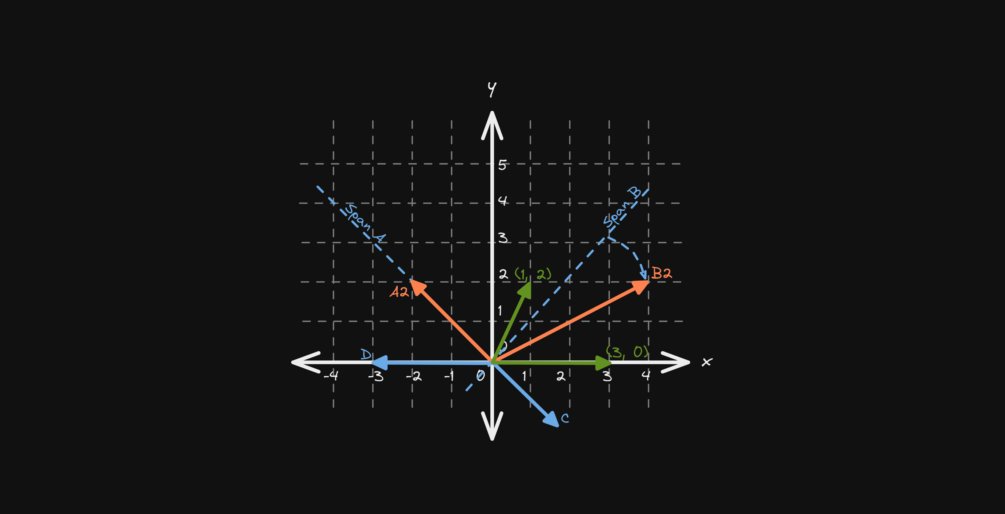
If we plot this transformation on a graph, it looks something like this

We can see that vector A1 has transformed into vector A2 along the same span - span A. But in the case of vector B1, it has transformed into vector B2 which has been pushed away from its original span - span B.
So for Matrix A, vector A2 is an Eigenvector. Also, when A1 transforms into A2, it scales by a factor of 2. This scaling factor is the Eigenvalue for Matrix A.
To summarise - Any vectors that remain on their original span after the transformation are the Eigenvectors and the factor by which they scale are the Eigenvalues of that matrix.
But since a matrix transforms an entire vector space and there could be an infinite number of vectors in that space, it implies that any vectors that coincide with the spans of these vectors are also the eigenvectors of Matrix A - as illustrated below.

When we plot the vectors of Matrix A (green vectors) on the graph, we observe that the first vector, with coordinates (3, 0), would also remain on the same span after the transformation, which is the X-axis. Hence it is also one of the eigenvectors of the Matrix.
Therefore, any vectors along span A and the X-axis, vectors C and D for example, are also the eigenvectors of Matrix A.
Use case
To put things into perspective, we can take a quick overview of one of the use cases of eigenvectors and eigenvalues without dwelling on too many details.
Imagine a cube in space, formed by a set of 3 vectors, which is rotated (transformed) by a 3D matrix by a certain degree.
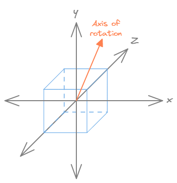
If you were to compute the eigenvector of that 3D matrix, what you would end up with is the axis of rotation. Since the rotation axis always remains on its span no matter the transformation. Also, rotation means there is no expansion or contraction of any kind and hence, the eigenvalue, in this case, is 1.
How to compute
To define the core concept symbolically, let us assume A is the transformation matrix and v is the eigenvector of that transformation. And since the transformation does not change the span of the eigenvector, it is the same as multiplying the eigenvector with some scalar quantity. This scalar quantity is the eigenvalue and it is represented by a λ. So the equation becomes.
$$A\vec{v} = \lambda \vec{v}$$
But fundamentally, we are equating a Matrix-vector multiplication with a scalar-vector product, which needs to be fixed.
To fix that, we can multiply λ with an Identity Matrix. This converts the RHS of the equation into a Matrix-vector product as shown here.
$$\begin{array}{} A\vec{v} = (\lambda I) \vec{v} \\ \text{where I is an identity matrix} \end{array}$$
Since we are solving for λ and v, we can subtract RHS from LHS and equate it to a zero vector. And then factor out the v.
$$\begin{array}{} A\vec{v} - (\lambda I) \vec{v} = \vec{0} \\ (A - \lambda I) \vec{v} = \vec{0} \\ \text{where } \vec{v} \text{ is a non-zero vector} \end{array}$$
The vector v needs to be non-zero otherwise it ends up having infinite solutions. So the only other way to satisfy this expression is when the product of the eigenvector v and the resultant matrix of (A - λI) equals zero. And as we have learned from the Determinants article, this is only possible if that matrix transforms the vector space into a lower dimension i.e. determinant of (A - λI) should be 0
$$\therefore |A - \lambda I| = 0$$
For the above expression, λ is the only unknown factor. This means that we need to find a value for λ such that when subtracted from A, the determinant of the resultant matrix is zero. This is best understood with an example.
Example
Find the eigenvectors and eigenvalues for Matrix A
$$A = \begin{bmatrix}{} 3 & 1 \\ 0 & 2 \end{bmatrix}$$
To find the eigenvalue, we know that the determinant of (A - λI) = 0
$$\begin{array}{l} |A - \lambda I| = 0 \\ \\ \begin{vmatrix}{} 3 - \lambda & 1 \\ \\ 0 & 2 - \lambda \end{vmatrix} = 0 \\ \\ (3 - \lambda)(2 - \lambda) - 1 \times 0 = 0 \\ \\ 6 - 3 \lambda - 2 \lambda + \lambda^2 = 0 \\ \\ \therefore \quad \lambda^2 - 5\lambda + 6 = 0 \end{array}$$
The resulting quadratic equation from the above calculations is known as the characteristic polynomial of Matrix A.
To find the possible values of λ, we know that the solution of a quadratic equation is given by...
$$\begin{array}{l} {-b \pm \sqrt{b^2-4ac} \over 2a} \\ \\ \therefore \quad \lambda = {5 \pm \sqrt{5^2-4 \cdot 1 \cdot 6} \over 2 \cdot 1} \\ \\ \qquad = 6/4 \text{ or } 4/2 \\ \\ \qquad = 3 \text{ or } 2 \end{array}$$
Let's substitute λ = 2 in (A - λI)v = 0, we get
$$\begin{array}{l} \begin{bmatrix}{} 3-2 & 1 \\ 0 & 2-2 \end{bmatrix} \begin{bmatrix}{} x \\ y \end{bmatrix} = \begin{bmatrix}{} 0 \\ 0 \end{bmatrix} \\ \\ \begin{bmatrix}{} 1 & 1 \\ 0 & 0 \end{bmatrix} \begin{bmatrix}{} x \\ y \end{bmatrix} = \begin{bmatrix}{} 0 \\ 0 \end{bmatrix} \\ \\ \therefore x + y = 0 \\ \\ \therefore x = -y \end{array}$$
If we assume an arbitrary value of x, say x = 1, then the vector with coordinates (1, -1) is the eigenvector of that Matrix A and as we know any vectors along the span of the eigenvector are also the eigenvectors of the matrix. So the equation x = -y is the equation of the span along which all the vectors are the solution for Matrix A
And of course, λ = 2 is the eigenvalue.
What do you think happens when we substitute λ = 3 in (A - λI)v = 0? Is the solution also an eigenvector? Try it out and leave your answers in the comments.
Special Cases
These are some special cases that are good to have at the back of your mind as they frequently appear in real-world analytics.
Shear Matrix
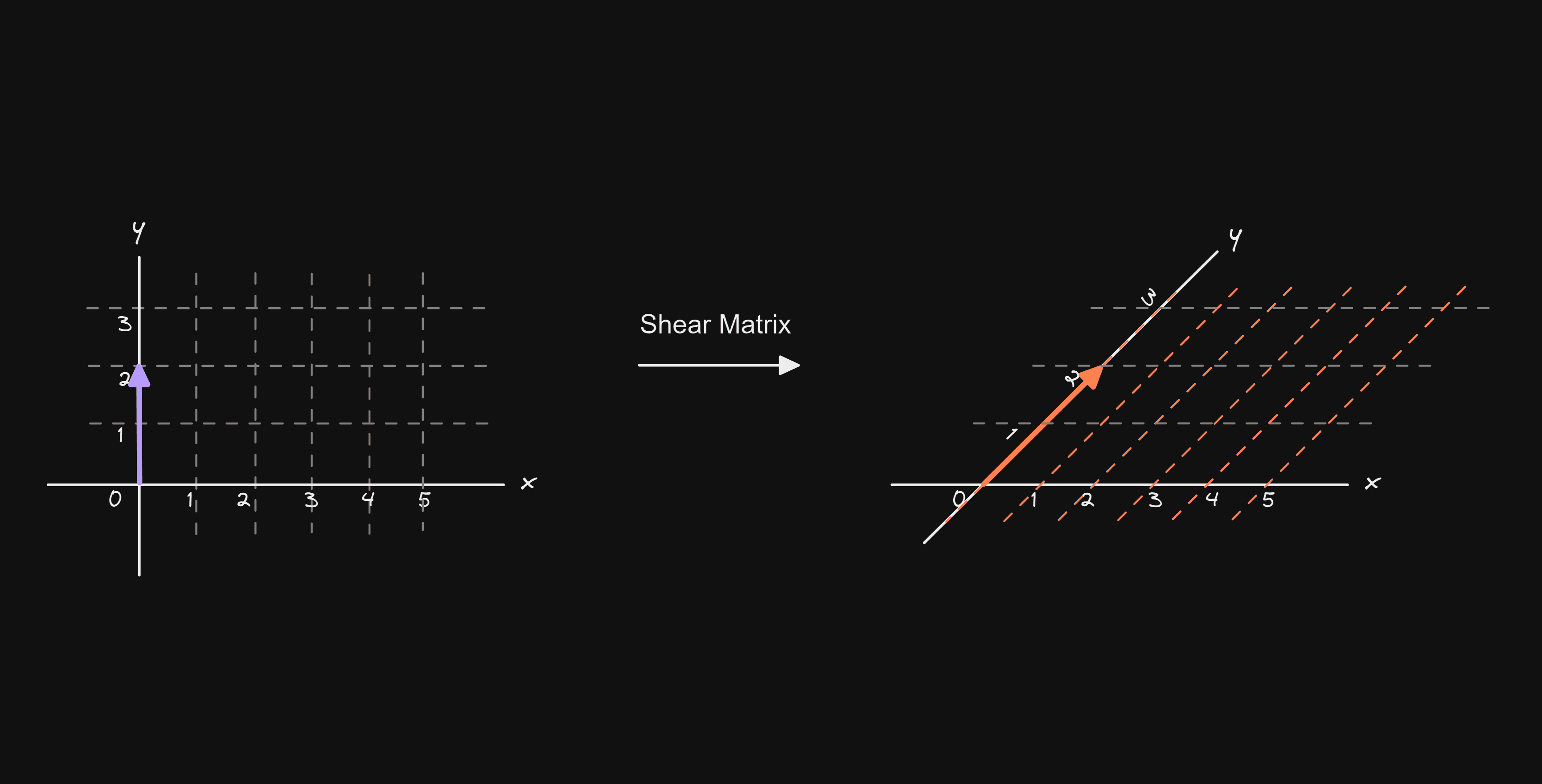
A shear matrix is a special matrix that only transforms either one of the two base axes (X or Y). In this case, we are going to consider a shear Matrix S - that transforms all vectors except the ones on the X-axis.
$$S = \begin{bmatrix}{} 1 & 1 \\ 0 & 1 \end{bmatrix}$$
Diagrammatically, it looks something like this
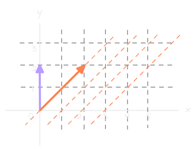
To find the eigenvector and eigenvalue first, we need to find the value of λ
$$\begin{array}{l} |S - \lambda I| = 0 \\ \\ \begin{vmatrix}{} 1 - \lambda & 1 \\ \\ 0 & 1 - \lambda \end{vmatrix} = 0 \\ \\ (1 - \lambda)(1 - \lambda) - 1 \times 0 = 0 \\ \\ (1 - \lambda)^2 = 0 \\ \\ \lambda^2 - 2\lambda + 1 = 0 \\ \\ \therefore \quad \lambda = 1 \\ \text{which is the only solution for this equation} \end{array}$$
Since the eigenvalue is 1 and we know that this shear matrix transforms all the vectors except the ones on the X-axis, we can say that all the vectors on the X-axis are the only eigenvectors for this matrix.
No eigenvectors and eigenvalues
A linear transformation may not have any eigenvectors and consecutively no eigenvalues. One such example is a matrix that only rotates the vector space by some degree. Say for example the following Matrix R
$$R = \begin{bmatrix}{} 0 & -1 \\ 1 & 0 \end{bmatrix}$$
It would be easier to understand why it cannot have any eigenvectors if we plot the transformation on a graph.

We can see that the orange vector leaves the X-axis and aligns with the Y-axis while the purple vector rotates off the Y-axis and aligns with the X-axis in the second quadrant.
So all that Matrix R really does is rotate the vector space by 90 degrees counter-clockwise, this means that any and all the vectors in the space shall also rotate off their spans. If no vectors remain on their span after the transformation then there can be no eigenvectors or eigenvalues for this matrix.
We can also prove this by attempting to calculate the eigenvalues for Matrix R.
$$\begin{array}{l} |R - \lambda I| = 0 \\ \\ \begin{vmatrix}{} 0 - \lambda & -1 \\ \\ 1 & 0 - \lambda \end{vmatrix} = 0 \\ \\ (0 - \lambda)(0 - \lambda) - (-1)(1) = 0 \\ \\ \lambda^2 + 1 = 0 \\ \\ \lambda = \sqrt{-1} \\ \\ \therefore \quad \lambda = i \quad \text{or} \quad \lambda = -i \\ \text{where } i \text{ is an imaginary number} \end{array}$$
Since the eigenvalues are imaginary numbers, there cannot be real eigenvectors
Bonus Tip
Although this is a shortcut to calculating eigenvalues, it only applies to 2D matrices. And anyway, if we are to find eigenvectors for 3D or higher dimensional matrices, we are better off computing them using a computer.
The trick to finding possible eigenvalues of a 2D matrix is
$$\lambda_1, \lambda_2 = m \pm \sqrt{m^2 - p}$$
Here, m is the mean of the first diagonal elements, and p is the determinant.
Let's try out an example. Find the eigenvalues for Matrix M
$$\begin{array}{l} M = \begin{bmatrix} 2 & 7 \\ 1 & 8 \end{bmatrix} \\ \\ m = {2 + 8 \over 2} = 5 \\ p = (2 \times 8) - (7 \times 1) = 9 \\ \\ \therefore \quad \lambda_1, \lambda_2 = 5 \pm \sqrt{5^2 - 9} = 5 \pm \sqrt{16} \\ \therefore \quad \lambda_1, \lambda_2 = 9, 1 \end{array}$$
Wasn't that quick?
Thanks for reading! If you think this article has helped you in any way or form, you can show your appreciation by reacting to this post and if you have any feedback, please leave them in the comments below.
Thanks again!
